Amplify Data Analytics with the Lighthouse Data Analytics model – Part 2 – CoE’s key functions

Part 2 of the Lighthouse Analytics Model, this post covers the Key Functions of the Data Analytics CoE. This is a rather short summary post, no need to spell out the details , rather highlight the key functions.

The Lighthouse Data Analytics Model at work in an organisation

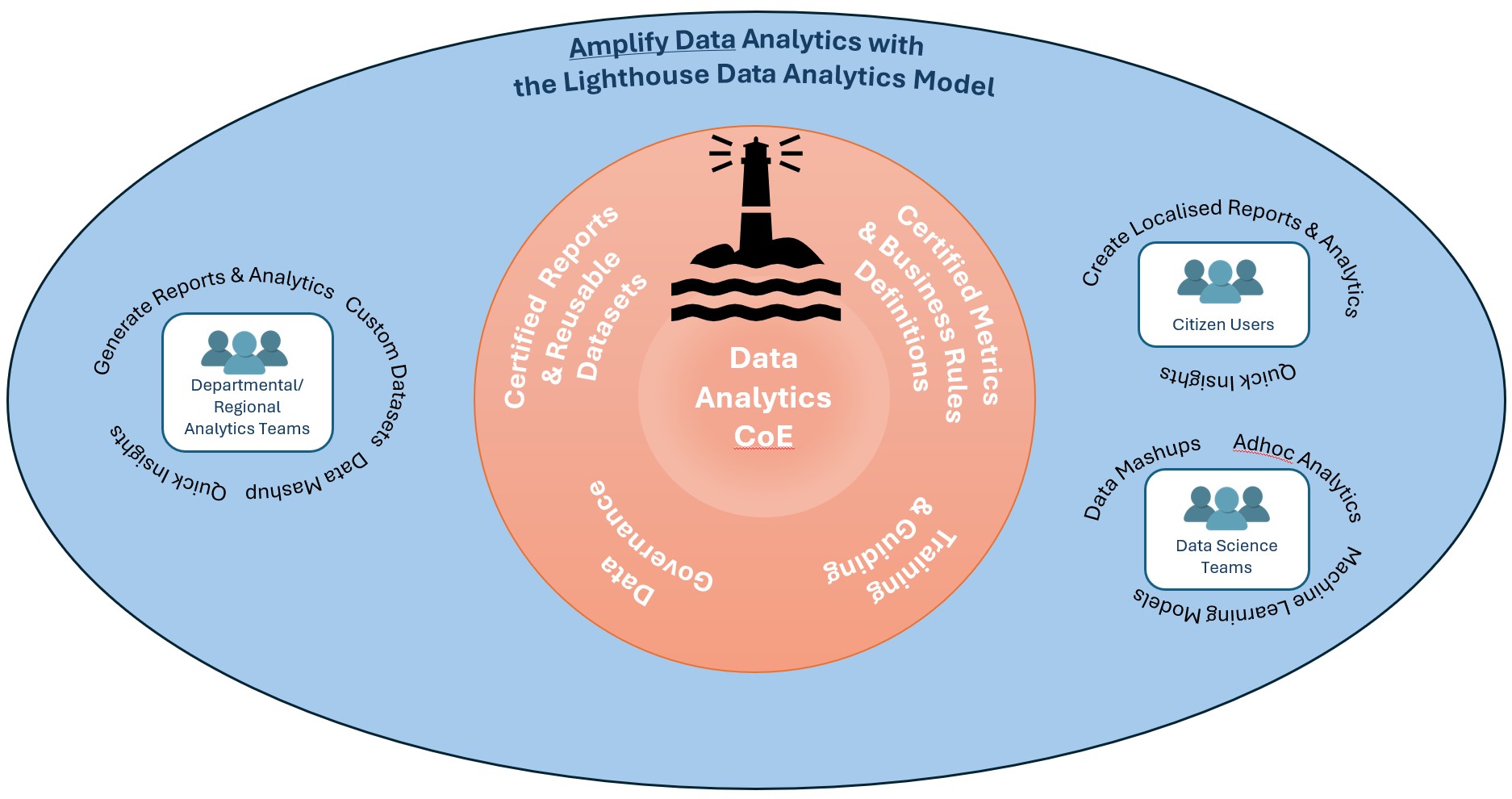
The Data Analytics CoE plays a pivotal role in organisations for Amplifying Data Analytics. It sets the path and guard rails on how departments & users can/should interact with Data for Data Analytics purposes.

Data Analytics CoE Key Functions

Key FunctionsInfo
Certified Metrics Produce key certified metrics for reuse-ability. These metrics are trusted by the organisation for accuracy and validity
Business Rules and DefinitionsOrganisation wide – clear, concise and consistent Business definitions and rules.
Resulting in reduced confusion and increased alignment.
Certified Reports/DashboardsPre-built Reports & Dashboards usable by authorized users / departments.
These provide the trusted data on key subject areas. It may not address all business questions however is geared towards providing access to the majority of key metrics.
Certified Reusable DatasetsHost Foundational Datasets usable by all departments. These are key for all complex and ad-hoc data analytics.
Power Users can reuse and further enrich these in their own workspaces.
End users utilise these for the majority of their ad-hoc analytics. These can be in the form of Databases and/or cubes.
AI/ML initiatives will also rely heavily on these certified datasets.
Data GovernanceGovernance scope is analytics assets only and not enterprise wide.
The policies, processes and practices established to ensure that data used for analytics is accurate, secure, and compliant with regulations. CoE would put these in place and audit them with an optional step of enforcement (if not handled by other departments).
Guard rails are established as part of governance to enable users flexibility but also restrictions on what they can or cannot do.
Training and GuidanceData Literacy is the key for amplifying analytics in organisations. Data Literacy requires ongoing training and guidance on what data is available but more importantly how to use and interact with data to answer business questions. Training programs are essential in building power users in the organisation who in turn will empower other users and increase the data literacy of the organisation.
Guidance refers to raising awareness of users responsibilities and how to work with data – this is a mix of training and governance.

The above are the core functions of what the Data Analytics CoE would perform in the Lighthouse Analytics Model, and hoping the above will aid in achieving the amplification of data analytics in the organisation.
Not going into much detail as most of these functions can be expanded easily by data experts, the objective of this post is to identify the key functions and its objectives .

Part 1 Amplify Data Analytics – Decentralise and embed into the business

Posted in Uncategorized | Tagged , , , , , | Leave a comment

Amplify Data Analytics – Decentralise and embed into the business

Intro

Data is the new water for today’s organisations. It is essential for their survival and growth, as it nourishes every aspect of their operations and strategy. It needs to flow to all users enabling them in making informed decisions and moving away from intuition and guesswork.
The challenge for many organisations has been in making data analytics accessible to all users.
How to enable the masses with curated & timely data analytics?
This blog post discusses this very topic and suggests a method on how to amplify data analytics in your organisation.

A Plan that created Noise and Kaos

It started with the Data Analytics vision – using data to drive greater insights, improving the business value, making data accessible to everyone and driving the data driven culture.
First step – setup a central dedicated specialist team to handle Data Consolidation, cleansing and enriching, and providing the Analytics. This team would help the organisation.
Great first step, but soon complains were surfacing from the business users around SLOW delivery, unable to help my department, when will my work get done, they do not understand what we want… and the list went on.
So what did go wrong? The central team consisted of the best Data Engineers, Modellers and BI Specialists, so why these complains?
Sound Familiar! This is the side effect of fully centralised analytics teams.

The Underlying Challenges of Centralised Teams

Centralised team models in large organisations frequently experience “delays” and mis-alignment with the business stakeholders. Why?

Central teams have single or very limited points of entry and output, these soon become bottlenecks causing large backlogs.
In turn resulting in the Central team having to prioritise work, with some work shifting to backlog (“delayed”) and some progressing ahead.
At this point noise from requesting departments increase. This noise starts a series of chain reactions – the department leaders with the loudest noise may get their work pushed forward at the expense of other works which could further slide back and cause more noise. The cycle continues.

The Bottleneck is the Central Analytics team.
Two options available at this point, further scale up the team and retain the same central model or move to a DECENTRALISED model.

The Decentralised Data Analytics Model

Note: Decentralised model in this postis not the same as Data Mesh?
Rather this is the first foundation step needed if Data Mesh is to be considered.

Whilst a Central Data Analytics team works very well for smaller organisations, that is not the case for larger organisations.
For larger organisations that suffer from centralised team fatigue, a stealth decentralised model commences to take shape. This model has a Central Data Analytics team and key departments running their own “lightweight” DA function, and in some rare cases, it is done with some central team’s guidance and collaboration.
This model scales up rapidly with all areas of the business, all departments are able to self-manage their own work, own targets and each able to scale up their lightweight DA team as needed. Lots of flexibility, but, this model does have its pitfalls and it can be very problematic if no controls are put in place.

The downsides of Decentralised models with no controls
With every department creating their own Analytics in silo, they are multiple drawbacks of this approach.

  1. Duplication of analytics, datasets and integrations across different DA teams
  2. there is zero or limited sharing, thus rework is high, leading to higher chance of discrepancies of the same metrics
  3. Inconsistent metrics
    • individual DA team’s may define a business metric with different logic or rules
      e.g. total sales from Marketing DA may be different to total sales from Operations DA team
  4. Inconsistent attribute & reporting
    • teams may decide to group attributes to how their department sees it rather than a consistent manner across the business.
      e.g. reporting of website sales as Digital whilst other team may show this as Online
  5. Lack of Data Governance and Compliance
  6. Teams would not be entirely across how data should be secured, or meet minimum regulatory requirements , e.g. GDPR

These and many other issues could promote the lack of trust in Data Analytics and also pose a high security & compliance risk.

A lot of challenges in an entirely distributed model, something is needed to connect all distributed pieces together, to guide them whilst allowing them to plot their own journeys.

An improvement would be to add the central Data Analytics Centre of Excellence (CoE) – “The Lighthouse”.

The Data Analytics Lighthouse

The Lighthouse Distributed Data Analytics Model

The Lighthouse Analytics model enhances on the fully distributed model by repurposing the Central Data Analytics/Business Intelligence team as THE LIGHTHOUSE (Data Analytics Centre of Excellence CoE).
In this model the Central DA team’s mandate is to provide overall DA Guidance/Training, manage Data Governance across all Data analytics and manage/provision ENDORSED reusable Data assets.

This central team ensures all Business Teams / Departments using and working with Data are:

  • Handling data in a safe and compliant manner
  • are aware of their data responsibilities
  • have adequate guidance on what they can or cannot do with data
  • trained on utilising and extracting value out of data
  • trained on utilising the Data Platforms to achieve their business objectives
  • aware of ENDORSED data assets that are maintained by the Central DA CoE
  • aware of global metrics and their definitions
The Lighthouse Data Analytics Model at work in an organisation

Next post I will cover the details of the LightHouse CoE core functions and how it engages with other departments and users.

Posted in Uncategorized | Tagged , , , , , | Leave a comment

Relative Period Modelling Part 2 – SSAS Multidimensional & ZERO MDX!

My second post of the Relative Period Modelling – detailing how to use the Relative Period database design in a SSAS (SQL Server Analysis Services) multidimensional cube. Remove the need to write a SINGLE MDX code for relative periods!

Note, this post assumes a good understanding of modelling with SSAS.

The first part, I detailed the database design of the Relative Period modelling – that design allows custom relative periods to be modeled and not be restricted by the relative period functions provided by the databases and SSAS. Please review that post if you have not already.

As with best practices of SSAS modelling (Multidimensional or Tabular), I am using VIEWS for the modelling rather than physical tables (Named Queries should also be avoided where possible) – done to avoid unnecessary cube rebuilds.

Note: I prefer to define all cube views in the cubefeed schema, allows the views to be isolated. 

Table View Description
DimDate cubefeed.DimDate Underling Date dimension view
DimDateSet cubefeed.RP_DimDateSet view over DimDateSet
DimComparativePeriod cubefeed.RP_DimComparativePeriod view over DimComparativePeriod
cubefeed.RP_FactDateSetDate view to represent date mapping as per DimDateSet
cubefeed.RP_FactComparativePeriodDate view to represent date mappings as per DimComparativePeriod
cubefeed.DimProduct using AdventureWorksDW2016
cubefeed.DimSalesTerritory using AdventureWorksDW2016
cubefeed.FactInternetSales using AdventureWorksDW2016

The RP prefix has been used to distinctively identify objects related to Relative Periods, this will assist in large models dealing with numerous facts.
(Dim Date based views have NOT been prefixed with RP_ to avoid confusing modelers)
Am utilising AdventureWorksDW2016 database for other facts/dimensions

SSAS Modelling with Relative Period

  • Create a new SSAS multidimensional database, called “RelativePeriods”
    Create a datasource and dsv.
  • Import all the view objects defined above into DSV and map as below:
    SSAS DSV
    Note: Relative Periods are kept isolated from other objects. They are linked in the cube via Dimension Usage – detailed later.
  • Dimensions
    Create the following dimensions (3 for Relative periods & 2 for the sample adventure works db)

    • DimDate
      This dimension is built off DimDate view, define hierarchies as needed.
      Ensure key is DateKey
      Dimensions DimDate
    • RP_ComparativePeriod
      a very simple one attribute dimension, using the similar named corresponding view created earlier (cubefeed.RP_DimComparativePeriod)
    • RP_DateSet
      a very simple one attribute dimension, using the similar named corresponding view created earlier (cubefeed.RP_DimDateSet)
    • Sales Territory
      Based off AdventureWorksDW2016 sample DB
    • Product
      Based off AdventureWorksDW2016 sample DBYou should now have the following dimensions in the project:
      SSAS Dimensions
  • Sales Cube
    time to create a sales cube that will bring the Sample Data and the Relative Periods
    together.
     

    • Create a new cube and label it Sales
    • Add Dimensions to cube
      Add all dimensions created previously
    • Mapped Date* needs some special handling, well not so special, simply add DimDate again and rename to Mapped Date.
      Ensure this dimension’s visibility is set to hidden
      * This dimension is responsible for linking all measure based facts using dates to the relative periods

    • Add Measure groups to cube
      Add the following measures groups/facts

      • RP Fact Date Set Date
        add only a count fact and set visibility to hidden
      • RP Fact Comparative Period Date
        add only a count fact and set visibility to hidden
      • Internet Sales
        added from AdventureWorksDW2016
        for simplicity only Sales Amount and Order Count measures are added 
    • The sales cube should now have the following, no MDX needs to be defined.
      SalesCube1_DimsandFacts
  • Dimension Usage – Linking it all together
    It is at this step where all pieces are linked together and the relative period process starts working for all facts.

    • Switch to the Dimension Usage tab
    • Link Product and Sales Territory dimensions to the Internet Sales measure group using ProductKey and SalesTerritoryKey respectively
    • Date dimension (not “mapped date”)
      • Link to “RelativePeriod Fact Date Set Date” & “RelativePeriod Fact Comparative Period Date” measure groups using DateKey.
        DimensionUsage_Date_to_DateSetDimensionUsage_Date_to_ComparativePeriod
      • Link Date dimension to “Internet Sales” using many to many via “RelativePeriod Fact Comparative Period Date”.
        DimensionUsage_Date_to_InternetSales
    • RP_DateSet
      • Link to “RelativePeriod Fact Date Set Date” using DateSet column.
        DimensionUsage_RP_DateSet_to_DateSet
      • Link to “RelativePeriod Fact Comparative Period Date” using Many to Many relationship via “RelativePeriod Fact Date Set Date”
        DimensionUsage_RP_DateSet_to_ComparativePeriod
      • Link to “Internet Sales” using Many to Many relationship via “RelativePeriod Fact Comparative Period Date”
        DimensionUsage_RP_DateSet_to_InternetSales
    • RP_ComparativePeriod
      • Link to “RelativePeriod Fact Comparative Period Date” using “Comparative Period” column
        DimensionUsage_RP_ComparativePeriod_to_ComparativePeriod
      • Link to “RelativePeriod Fact Date Set Date” using Many to Many relationship via “RelativePeriod Fact Comparative Period Date”
        DimensionUsage_RP_ComparativePeriod_to_DateSet
      • Link to “Internet Sales” using Many to Many relationship via “RelativePeriod Fact Comparative Period Date”
        DimensionUsage_RP_ComparativePeriod_to_InternetSales
    • Mapped Date – key date dimension that joins to other facts
      • Link to “RelativePeriod Fact Comparative Period Date” using DateKey and MappedDateKey.
        DimensionUsage_MappedDate_to_ComparativePeriod
      • Link to “RelativePeriod Fact Date Set Date” using Many to Many relationship via “RelativePeriod Fact Comparative Period Date”
        DimensionUsage_MappedDate_to_DateSet
      • Link to “Internet Sales” using DateKey and OrderDateKey
        DimensionUsage_MappedDate_to_InternetSales
      • Future facts are all to join to the Mapped Date dimension using DateKey

  • The final Dimension Usage matrix should look like below:
    DimensionUsage_Overall


Update Data & Deploy Model 

Modelling is now complete,
Since most of the relative dates configured is in the current period, whilst the AdventureWorksDW2016 database is using periods in 2016 and prior.
To allow testing, you have two options:

  1. Update a subset of AdventureWorks database dates to being more recent
  2. or Change the RelativePeriods to be in history

Will leave the decision to you, personally I have opted for option 1, allowing me to test relativeperiods using current dates.

Once data is updated, deploy model and ensure it is built and processed successfully.

Connect via Excel & Test

Lets connect via Excel and test if the relative period model actually works or not.

  1. Test Comparative Periods in Excel
    1. Bring Dates to rows and Comparative Period dimension to columns
    2. Drag in Internet Sales Amount in measures
    3. The Default node in Comparative Period dimension always returns the measure without any comparative period calculations being applied. Use the Default node to test whether comparative period calculations are working or not.
      See below output:
      Excel_ComparativePeriods
    4. Comparative Periods is working!!!
      Compare last year values to the corresponding prior year values under default and notice how they are matching!
      Similar checks can be done for Last week and yesterday.
    5. You can further test this by adding new Comparative periods in dimensions and facts, such as last 2 days back etc, reprocess the cube (no need to deploy) and these will now simply appear and work.
    6. Similarly, bring DateSet dimension to the filters are and select a DateSet, the dataset in Excel will change to the constant period selected. In my case I selected “Last4CompletedWeeks”,which causes the rows to show the last 4 weeks – notice how the Date dimension on the row has no filters applied and yet is only showing last 4 weeks with data!
      Excel_DateSets

We now have a completely data driven relative period model, no need to perform complex MDX logic, simply insert the DateSets and/or Comparative Periods in the respective Dimensions and Facts and you have these relative periods working. You can make these relative period as simple or as complex as required – all that is needed is a good handle of SQL and ZERO MDX!

Hope you find this useful.

Posted in Uncategorized | Leave a comment

Relative Period modelling for multiple platforms

There are a lot of write-ups on relative periods, and different methods exist for a variety of tools. Interestingly each platform requires special handling, e.g. COGNOS Transformer & TM1 handles relative periods differently to SSAS multidimensional, and again differently to SSAS Tabular, than you have paginated reporting tools such as SSRS, Crystal reports, BO when reading directly off a database, they need another method to handle relative periods, and soon we end up maintaining a few methods to handle the same relative period logic.
Add to that additional complexity if your organisation uses a CUSTOM date calendar, in which case not all of the builtin functions for the platforms may work!!

I have been on a similar journey with my current company, using COGNOS Transformer, SSAS multidimensional, SSAS tabular, SSRS & Power BI, and ended up managing multiple methods of maintaining relative period logic. Each platform requiring something slightly different, and worse, if rolling out new relative period calculations, the rollout process would be lengthy and error prone! Plus the organisation uses a CUSTOM date calendar, so most of the builtin MDX functions like ParallelPeriods are no good :(.

Looking for a better way to manage this, I came up with a data model that I believe could be maintained centrally and accessed by multiple platforms for relative periods .

The design consists of the following:

  • Relative Periods modeled in a database (central foundation piece)
    This model will consist of the Date dimension which will mirror the organisations calendar.
  • Using the foundation database objects, incorporate these in the relevant tools, e.g. SSAS multidimensional, SSAS tabular, SSRS etc….
  • Any relative period changes or addition of new periods are applied to the central foundation database model, and as long as the tools have incorporated these objects correctly, they will all be able to use the new periods easily.


Relative Periods Database Model

Relative Periods foundation database model

The foundation database model for the relative period design

The database model consists of the following tables/views:

  • DimDateSet
    a dateset defines the constant relative periods, e.g. Today, Yesterday, Current Week, for these relative periods, there are only a constant set of dates on a daily basis.
    no dates are specified here, only the dateset names.
    Sample contents below:
    sample_dimdateset
  • DimDate
    the traditional date dimension, here you would define the calendar as required by the organisation. The Primary key is the DateKey which is in the format YYYYMMDD
    Note: Except for RelativePeriod Facts, no Fact table should join to this dimension
    Sample contents below:
    sample_dimdate
  • DimMappedDate
    role playing dimension, this is a view based on DimDate and only exposing the DateKey.
    all facts with measures are mapped to this dimension.
  • DimComparativePeriod
    relative periods where a comparison is done for a selected date, these are different to datesets, that are constant. e.g. for any given date, show the same day Last week, or same day Last year etc. No dates are specified here, only the comparative period names.
    Sample contents below:

    sample_dimcomparativeperiod
  • FactDateSetDate
    factless fact that bridges DimDateSet and DimDate. It is in this object, where the Datesets are mapped to the corresponding Datekeys. Since the dates for each dateset will change daily, this object could be a view consisting of multiple UNION select statements (one for each Dateset). Else if performance is essential, than this could be stored as a table (you will need to have a refresh process to update this daily)
    Sample contents below:
    sample_factdatesetdate
  • FactComparativePeriodDate
    factless fact table bridges DimDate, DimComparativePeriod & DimMappedDate.
    for each comparativeperiod, all datekeys from DimDate are mapped to a corresponding MappedDateKey,
    e.g. for comparative period Last Week, all dates from the DateDimension are mapped to the corresponding date 7 days back.
    Sample contents below:
    sample_factcomparativeperioddate


These database objects are related as below:

Relative Periods foundation database model

The foundational database model for the relative period design

With the above database model in place, you can now use that in any reporting platform to build your relative periods as needed.
My next post will walk through how to use this in SSAS dimensional & tabular models.


Posted in Uncategorized | 1 Comment

COGNOS Cube reports–slow performance

This week, I took on optimising a cube report which I had authored recently. This was a not too complex burst report working off an SSAS 2008 cube. The report was taking around 1 minute per burst, with around 500 bursts required = 500 minutes (over 8 hours).

The issue in my report was the use of Detail and Summary filters. Whilst they do work, the effect they have on an OLAP data source is significant!

Inspecting the MDX generated by Report Studio, showed lots of UNIONS, AND CROSS JOINS. What was occurring – Report Studio was performing full cross joins and then applying the detail and summary filters to the returned record set.
In this case, the cross joins resulted in a record set that could easily surpass 100 million records!!! Even though the end result was correct, this was adding a significant overhead to the report.

Remember; COGNOS firstly performs a cross join between all query members and then applies the summary and detail filters

How to optimise this – SIMPLE, reduce the resultant cross join result set, which would require the use dimensional functions within the Query members, e.g.
previously whilst I had the entire member level, now I had
FILTER ( {set}, {condition})

using the above, I was able to limit my query members to the select few records, which also meant my record sets were significantly smaller.
In the end, I was able to totally remove the Detail and Summary filters and the bursting now takes around 5 seconds each!! not a bad outcome, from over 8 hours to 40 minutes!

As a simple rule, avoid using Detail and Summary filters on dimensional reports.

Posted in Uncategorized | Leave a comment

COGNOS 10 Upgrade from 8.3

Currently in the process of performing a COGNOS BI upgrade from 8.3 to 10.1.

Instead of performing a big bang approach upgrade on the existing server, have deployed a new server, and performed a clean install of 10.1. Setup the new 10 environment – we now have two COGNOS environment 8.3 & 10. Once setup, imported the entire 8.3 package (which I had previously exported from 8.3) into 10. Walla – all my reports are packages appear as there were in 10. One major task to remember – it has brought along all schedules – the first step post import, is to use the new COGNOS 10 Schedule suspend feature and suspend all schedules for the day and maybe for the next few days whilst all testing is performed. Alternatively you could disable all schedules

Have found a few of the dimensional reports are failing with strange error messages – shall post the error messages 2morrow.

NO MORE CUBE SWAP….. with 10 (and 8.4 I think) transformer now takes care ofh swapping cubes, by using a MDC file pointer that points to the current MDC file, and even better is the ability for it to delete old version – you can specify the number of versions to retain – finally a very much needed enhancement.
Transformer login with multiple namespaces works  – always had issues in 8.3, where autologin to namespaces would fail, seems to be working fine with no issues at all on 10.
Transformer speed improvement!!! it now uses the available memory to build cubes in RAM rather than disk I/O. The reduction in cube build times is very noticable. In a couple of cases, my cubes builds have gone from 26 minutes to 4 minutes!!!

I still reckon SQL Analysis Services build faster cubes!!

Posted in Uncategorized | Tagged , , , | Leave a comment

About me

My name is Dharmesh Kalyan, and I am Data Professional loving all things Data and Business Intelligence. Have been working with Data for a number of years from small analytical databases to large scale Data Lakes and Data warehouses supporting large scale Global Analytical solutions.
SQL is what I work with and love.
Technologies I love – SQL, Analysis Services, MDX, Power BI, DAX, SQL Server & Snowflake.

Some key things I follow in my professional life:

  • listen more and speak last
  • KISS – Keep it simple stupid
    the simple things in life are often the best , this also applies to technology solutions!
  • It always seems impossible until it is done – Nelson Mandela
  • Never start any work until you know what you trying to solve
    ….and never write a single line of code until you have a design / data flow 
  • WE is better then I or ME

Residing in Brisbane Australia, and been in the Data industry for over 25 years.

I am currently employed as Group Head of Data at Domino’s Pizza Enterprises, but the statements and views expressed here are mine alone.

Feel free to connect with me on LinkedIn

Posted in Uncategorized | Leave a comment